Part 3: Can AI extract planning data from zoning by-laws accurately?
In Part 1 of this three-part blog post series on whether AI can accurately extract planning data from zoning by-laws, Esri Canada GIS analyst Jocelyn Tang introduced the problem and examined different LLMs in search of the right model for the task. In Part 2, she explored different metrics to use when evaluating LLMs. She also concluded that using LLMs as a tool for extracting information from Zoning By-laws has an accuracy of around 70%. Now, in the final part of the series, Jocelyn concludes her investigation by fine-tuning one of the models she used in Part 2 to see whether it might improve the results.
Encoder-only models need further domain specific fine-tuning to see improvements in accuracy. In Part 3 of this blog post series, I want to explore fine-tuning and see if I can improve the F1 score of the best-performing pre-trained question-answering model identified in Part 2 (Robustly Optimized BERT Approach or RoBERTa) by fine-tuning it to zoning by-law text.-
Fine-tuning versus pre-training
It is easy to assume that there is one way to train AI models. In fact, there are many different types of training methodologies. It is important to understand the difference between fine-tuning a model and pre-training a base or foundation model from scratch.
Pre-training: This is the initial phase of training an LLM, where the model has no prior knowledge. The goal of pre-training is to create a foundational base model that understands general language (for example: GPT, Claude, RoBERTa and BERT). The LLM is trained on a large, diverse dataset (often billions and trillions of tokens made of data from the Internet, books and code) to develop a broad understanding of language, context and various types of knowledge. It is computationally expensive and involves massive amounts of data.
Fine-tuning: Fine-tuning is taking an already pre-trained base model and further training it on a more specific dataset. The datasets used in fine-tuning are often domain specific. This is so that the fine-tuned model can perform better on specific tasks or scenarios that were not well covered in pre-training, for example: medical diagnoses, specific legal texts or documents. Fine-tuning aims to enhance an existing model’s knowledge in specific contexts rather than expanding its general knowledge. It is less computationally expensive and requires a much smaller dataset than pre-training.
Zoning by-laws are a domain-specific dataset and in this scenario, it makes sense to fine-tune an existing pre-trained model!
For further reading on this topic, consult IBM’s documentation on fine-tuning.
Fine-tuning methodologies
There are many different ways to fine-tune a model. In this blog post, I’ll only cover a few key methodologies.
Supervised fine-tuning (SFT): This is the simplest method of fine-tuning and works best for well-defined tasks. It involves a dataset of pairs of inputs and outputs. The model takes the input and produces the desired outputs like classification labels or continuations of a prompt. Dataset preparation is critical.
Parameter-efficient fine-tuning (PEFT): A major challenge with fine-tuning LLMs is their size. Normally, fine-tuning re-trains all the parameters in the model. PEFT only fine-tunes a small portion of the model’s parameters. This drastically reduces resource requirements. (An example of a tool that provides infrastructure to fine-tune your LLM is DigitalOcean.)
In the case of fine-tuning an existing pre-trained RoBERTa QA model to zoning by-law data, I chose supervised fine-tuning as my approach.
For further reading on LLM training, consult
Understanding learning curves
Before proceeding to fine-tune the model, it is important to understand learning curves. Learning curves help you evaluate the model’s performance during training and identify potential issues before they reduce performance.-
Loss curves show how the model’s error (loss) changes over training steps-.
Accuracy curves show the percentage of correct predictions over training steps.
And validation loss curves are metrics that evaluate a deep learning model's performance on a validation dataset (a set of data that the model has never seen during training)-.
Could re-word it as "DigitalOcean provides the infrastructure to allow you to host and fine-tune your LLMs". But my original intention wasn't to sell another company's product but more like acknowledge where the information came from.
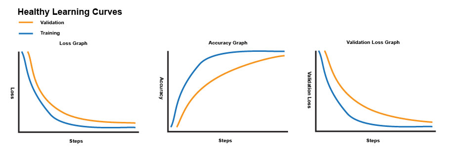
Examples of what healthy loss, accuracy and validation curves look like as a graph.
The model should start with high initial loss before training because predictions are initially poor. As training progresses, the loss should generally decrease. Eventually this stabilizes at a low value as the model has learned the patterns in the data.-
For accuracy curves, the initial accuracy should be low and as the training progresses, it should improve as the model learns the patterns of the data. Accuracy curves may show plateaus as the model makes predictions closer to the desired and correct answer.
For further reading on learning curves, consult Hugging Face’s LLM course and GeeksforGeeks’s sheet on training and validation loss in deep learning.
Preparing the training dataset
As mentioned earlier, dataset preparation is critical for domain specific supervised fine-tuning. Datasets must be cleaned and formatted in a way the model can consume. For more information regarding dataset preparation, refer to part 2.
For this project, I conducted two fine-tuning experiments and used a training dataset of 100 and 500 labelled examples.
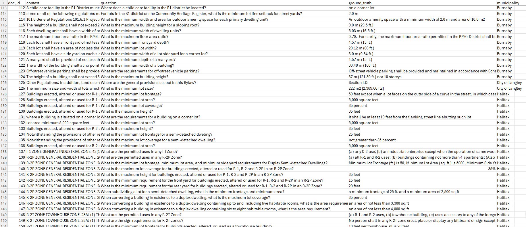
Screenshot of a snippet of the training dataset used.
What were the results of the fine-tuning?
Below is an image showing the training and validation loss summary for the 100- and 500-sample training dataset fine-tuning experiments.
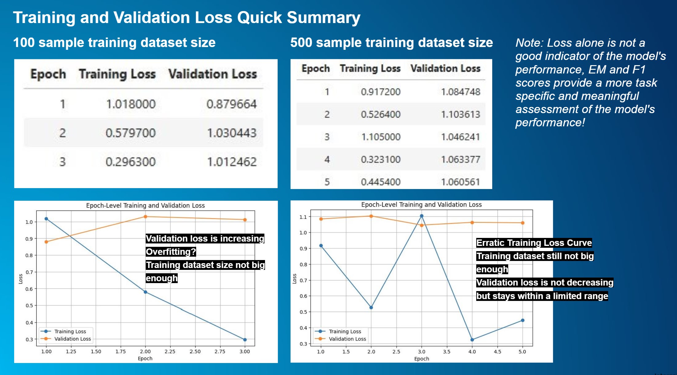
An image showing the training and validation loss summary for the 100 and 500 sample training dataset fine-tuning experiments I ran in this blog post.
Below is a table showing the metric EM and F1 scores (for definitions of what these metric scores mean, refer to Part 2 in this blog post series) for the 100- and 500-sample training dataset fine-tuning experiments.
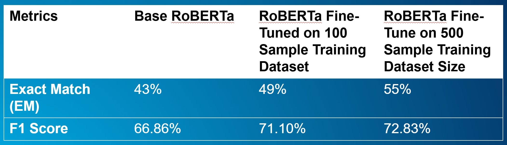
Note: Loss alone is not a good indicator of the model’s performance. EM and F1 scores provide a more task-specific and meaningful assessment!
One thing I discovered when learning about learning curves is that tutorials give students ideal examples. In reality, training and validation loss numbers often show fluctuations, especially with small training dataset sizes! Don’t be surprised when conducting early experiments to find it challenging to interpret graphs and numbers.
In both experiments, training loss generally decreases at a stable rate except for a random fluctuation and increase in epoch 3 of the 500-sample experiment. However, the validation loss increases in the 100-sample experiment and does not improve much in the 500-sample experiment. It stays within the same range. This might be due to the small training dataset size.-
What I learned is that loss alone is not a good indicator of the model's performance and EM and F1 scores, especially for question answering, provide a more meaningful assessment. So, I focused more on those metrics instead.-
Compared to the base model, fine-tuning with the 100-sample training dataset works with a +12 EM improvement and around a +6 F1 improvement. However, for the 500-sample training dataset, there is only around a +1 EM and F1 gain. Between the 500-sample-trained model and the 100-sample model, there are diminishing returns.-
It also appears that after fine-tuning, models still struggle to answer challenging questions and cannot return answers that have lots of conditional statements and long sentences. Below is a screenshot of some responses the model returned during evaluation after training:
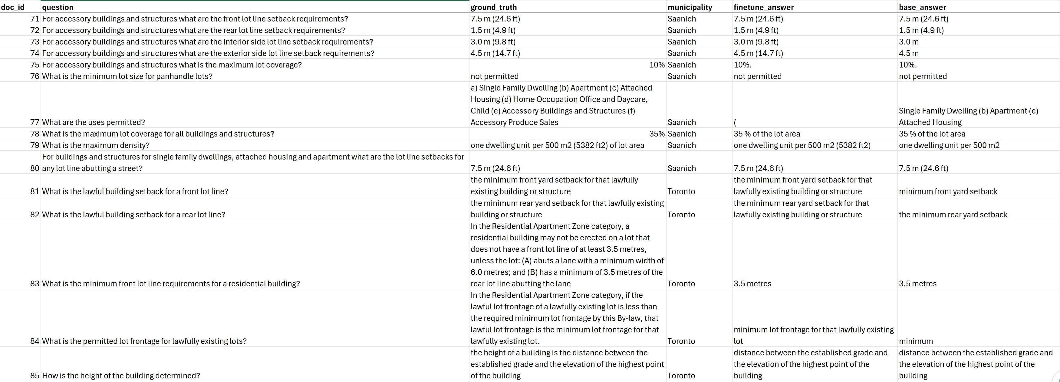
A screenshot of some responses the model returned during evaluation after training.
There may be a few possible reasons why there are diminishing returns:-
- Most of the gain came from 100–200 data examples-
- The domain might not be so different and maybe fine-tuning isn’t the right solution
- The dataset is not big enough in relation to the model size (explains the very erratic training loss graph)-
- Maybe a more diverse or challenging dataset would help with more varied and ambiguous questions with tricky wording- (this is unlikely because I made sure to include a good variation of easy and difficult questions and answers)
- Wrong choice of training arguments/hyperparameters
If you’re interested in looking at the source code and workflow, check out the Github repository for this project.
Concluding thoughts
I believe the reason for diminishing returns in the model’s accuracy is because the dataset is not big enough in relation to the model size. To achieve further improvements in accuracy, I would probably need a dataset of 10,000 + examples instead of the current 500!
To sum up my whole journey, I considered the project to be a success in that I learned a lot in the process despite not achieving ideal results. If you recall, in part 1 I stated that this blog post series aims to share my learning journey by breaking down technical concepts into an easy-to-understand way.
Finally, it is important to remember what urban planning is about: creating thriving communities for everyone. Great urban planning is about creating a sense of belonging and a sense of place. It requires balancing not only tangible factors like land use, transportation and infrastructure, but also intangible considerations such as culture, identity, equity and community values.- This requires human empathy, judgment and local knowledge. As I’ve shown in part 3 above, the model isn’t ready to be run without a significant amount of human judgment in the mix, so be sure to take caution when using LLMs to process zoning data and check your work.
In general, when using AI tools…
- We need to think critically about their output
- We need to be aware of the biases and the quality of their training data and algorithms
- We need to understand the strengths and limitations of different AI tools and types of models
- We need to continuously evaluate the accuracy of these technologies to ensure they support the desired outcomes, especially for high-risk tasks and decision-making processes
We must remember that AI technologies are tools and it should be humans in the driver’s seat.
Continue the conversation by joining our LinkedIn group.