Map urban change: ArcGIS workflows for built environment change detection

Change is constant— Cities evolve, landscapes shift and infrastructure transforms. Understanding these changes is vital for smart planning and sustainable development. In this post, I walk through two practical imagery workflows in ArcGIS Pro to detect changes in the built environment, identifying new development and built loss over time.

Change detection is the process of identifying differences in a place or landscape by comparing data collected at different times to answer questions such as: What changed? Where? When? By how much? Detecting change in the urban built environment means identifying how human-made structures, such as buildings, barren lands, roads and other infrastructure, expand, shrink or transform over time. Unlike vegetation or natural landscapes, built features have distinct spatial and spectral patterns that make it possible to map and monitor surrounding non-built areas. Understanding these changes is important because the built environment directly shapes how people live, commute and interact with their cities.

In this post, I’ll walk through two ArcGIS imagery workflows for detecting changes in the built environment. The analysis uses PlanetScope imagery, which provides 8 spectral bands at approximately 4.7-meter resolution. For demonstration, we’ll compare images from June 2023 and June 2024 over Gatineau, Canada. By the end, you’ll have a clear understanding of the primary tools available in ArcGIS for built environment change detection and how to choose the right method for your project, depending on your goals and the imagery you’re working with.

Pixel-based change detection

Pixel-based change detection compares pixel values between two raster datasets to highlight changes over time. In the context of the built environment, this method is especially useful for detecting where new construction has occurred or where built-up areas have been removed. Instead of classifying land cover directly, it focuses on the magnitude and direction of pixel value differences between two dates. Here’s how to apply a pixel-based change detection of the built environment in ArcGIS Pro:

Step 1. Calculate NDBI for each image

The Normalized Difference Built-up Index (NDBI) emphasizes urban features by comparing the reflectance of built surfaces in near-infrared (NIR) and shortwave-infrared (SWIR) bands:

As PlanetScope imagery does not include a true SWIR band, we approximated NDBI using Band 4 (Red) and Band 8 (NIR). This ratio-based index helps minimize the effects of atmospheric conditions and illumination differences. Follow the steps below and calculate NDBI for both images: 

Calculating the NDBI for image Time 1 (June 2023) 

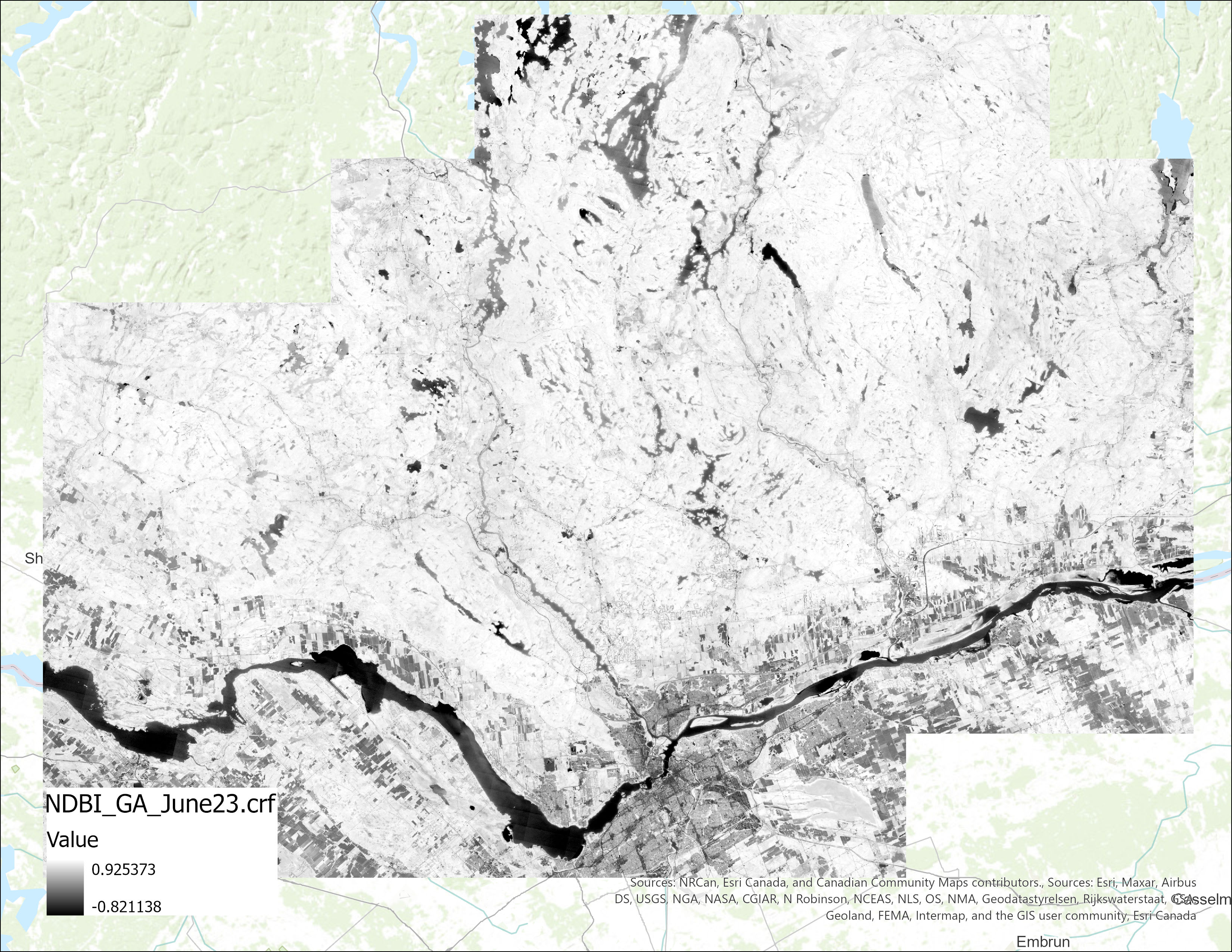
Created single-band NDBI raster for image Time 1 (June 2023)

Step 2. Normalize pixel values

To account for atmospheric or sensor-related inconsistencies, normalize the pixel values using the Raster Calculator. Below is the formula used for normalizing the NDBI raters based on raster’s Mean and Standard Deviation:

You can retrieve the Mean and Standard Deviation from the raster’s symbology:

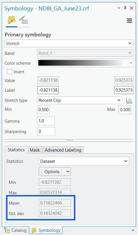
Retrieving the Mean and Standard Deviation values from NDBI raster’s Symbology pane

Use the tool and the following settings to apply this process to both the 2023 and 2024 images to ensure comparability:

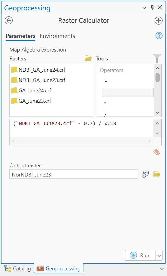
Using Raster Calculator tool to normalize both NDBI rasters

Repeat step 1 and 2 for the image Time 2.

Step 3. Run the Change Detection Wizard

There are different ways you can apply pixel-based change detection in ArcGIS Pro. Change Detection Wizard is one of them. This tool requires the Image Analyst extension and works in a 2D map scene. In this step, follow the steps in the video below to apply Change Detection Wizard using the two normalized NDBI rasters for Time 1 and Time 2 (June 2023 and June 2024). 

Running Change Detection Wizard (pixel-based method) using the two normalized NDBI rasters

In the Classify Difference step, adjust the histogram ranges until the categories represent meaningful thresholds of change for your imagery.

The final output raster highlights built gain (areas newly developed in Time 2), built loss (areas where built features disappeared in Time 2) and no change (stable areas with little or no difference between Time 1 and 2).

Pixel-based change detection result: June 2023 image (left), June 2024 image (middle), and change detection raster (right) where green pixels show built environment gain and red pixels represent built environment loss. 

Categorical change detection

Categorical change detection focuses on identifying transitions between classes, such as land cover types, over time. Unlike pixel-based methods, which analyze raw spectral values, categorical workflows classify imagery into thematic categories (e.g., Built, Green, Water) and then track how those categories change. This makes it especially useful for mapping broad land cover dynamics and producing easy-to-interpret outputs.

In this workflow, we’ll classify each image separately and then compare them using ArcGIS Pro’s Change Detection Wizard.

Step 1. Perform unsupervised classification

Perform an unsupervised classification on both raw images using Iso Cluster Unsupervised Classification tool and following the steps below:

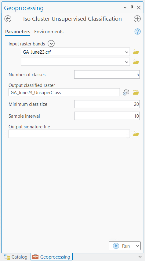
Performing unsupervised classification on image Time 1 (June 2023) using Iso Cluster Unsupervised Classification tool

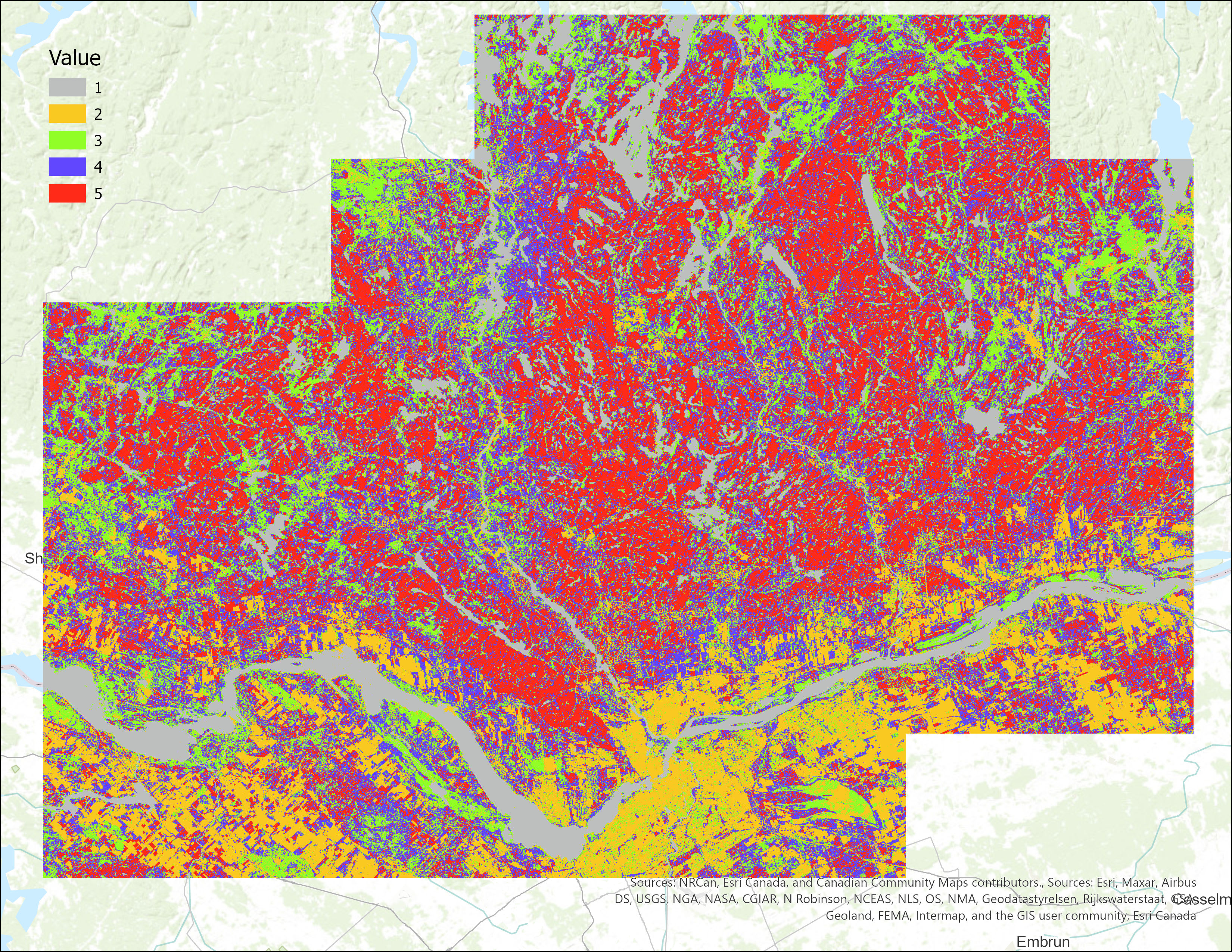
Unsupervised classification raster result

Upon inspection, you’ll notice each class aligns with ground features. In this example, here are the features each class represents:

• Class 1: Waterbodies

• Class 2: Built environment (roads, rooftops, infrastructure)

• Classes 3–5: Vegetation

Comparing the unsupervised classification result with the actual image to evaluate how classes represent real-world features

Using this logic, we combine vegetation classes into a single category in the next step. This simplifies the dataset into meaningful categories.

Step 2. Reclassify into final categories

Apply the Reclassify tool to both rasters to reduce the number of classes into cleaner thematic rasters. For this workflow, we reclassify into three categories: Water, Built, and Vegetation.

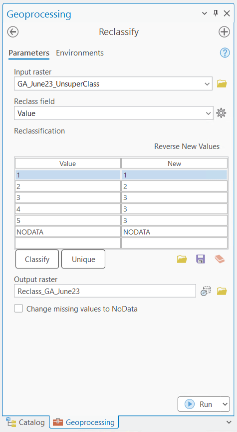
Using the Reclassify tool to aggregate the classes from 5 to 3

Comparing the reclassification result with the actual imagery to make sure the new classes represent the real-world features well

Repeat step 1 and 2 for the image Time 2.

Step 3. Run the Change Detection Wizard

Now, launch the Change Detection Wizard and select the Categorical Change option using the steps below:

Running Change Detection Wizard (categorical method) using the two classified rasters

During the Output Generation step, you might need to adjust post-processing settings based on your imagery types and classification results:

• Smoothing Neighborhood: helps reduce noise in classified rasters.

• Statistics Fill Method: fills in small gaps to produce a cleaner map of categorical changes.

The output highlights transitions such as Water to Built, Water to Vegetation, Built to Water, etc. Now, you have a categorical change map that clearly shows how different land cover classes transitioned between Time 1 and 2.

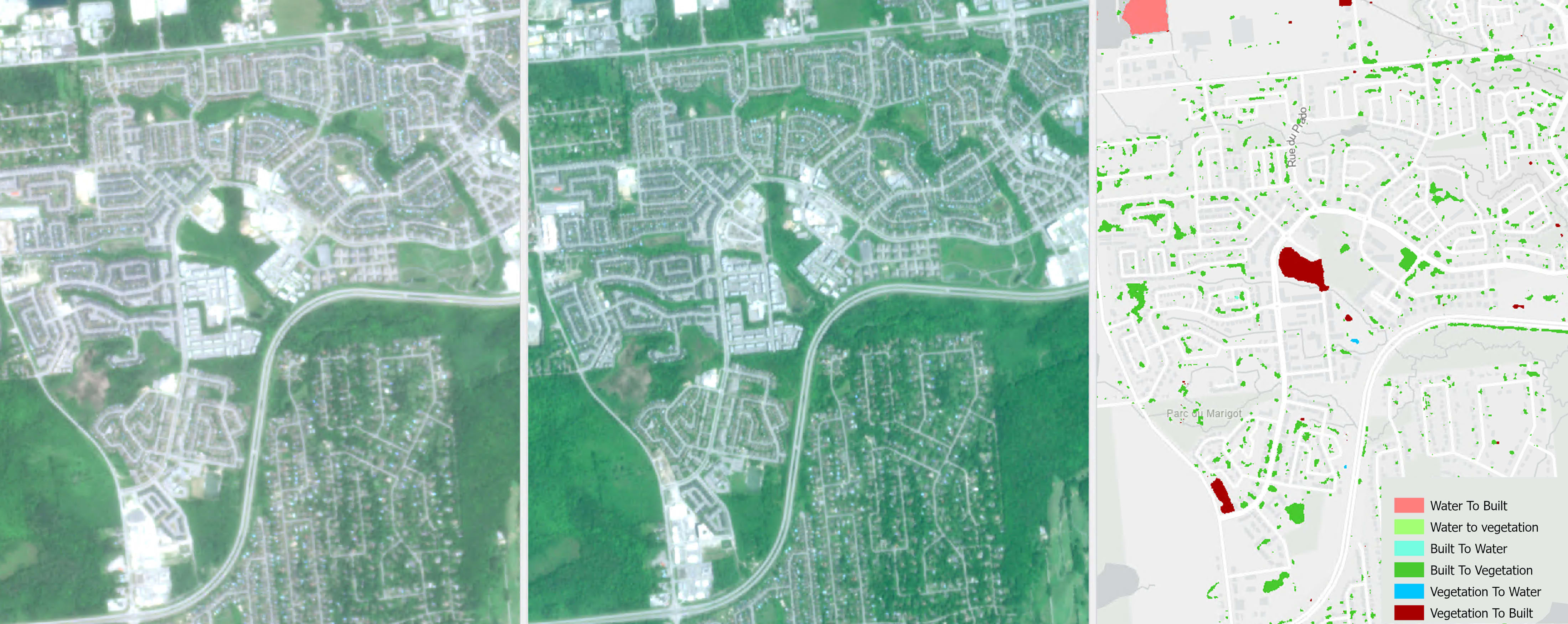
Categorical change detection result: June 2023 image (left), June 2024 image (middle), and change detection raster (right) where transition categories are shown. 

Tip: You can replace the unsupervised classification in Step 1 with a supervised classification if you have training data or want more control over class definitions.

Conclusion

Detecting change in the built environment is essential for understanding how cities grow, adapt and respond to pressures like population growth, climate impacts or disasters. With imagery and the powerful analysis tools in ArcGIS Pro, you can transform raw pixels into actionable insights. In this post, we explored two workflows:

• Pixel-based change detection, which highlights spectral differences and is well-suited for quickly spotting subtle changes.

• Categorical change detection, which tracks transitions between land cover classes and produces easy-to-interpret thematic maps.

Each approach has its own strengths, choosing the right one depends on your project goals, data type and audience. For urban planners, infrastructure managers and researchers, these workflows provide practical, scalable methods to monitor change and support informed decision-making.